2021-04-09

Monte Carlo Integration

In high school, we were taught how to do simple integrals like $$\int 4 x^3 + \frac{1}{9} x^2 \, \mathrm{d}x$$ by hand. But what about more complicated integrals like $$\int e^x \sin x \, \mathrm{d}x?$$ If you know how to do integration by parts then you can calculate the integral to be $$\int e^x \sin x \, dx = \frac{e^x}{2}(\sin x - \cos x) + C$$ for some constant $C$. But what about even more complicated integrals, like multi-dimensional integrals, or integrals for which no closed form solution exists. What do you do then? In some cases you can slog it out and maybe eventually, after many hours of study and perseverance, find a formula for the integral. But in many cases all you can do is simplify the integral into terms containing other simpler integrals. After that you have to resort to numerical integration techniques to make further progress on the problem that you are working on.

However, in many cases, a numerical solution is all that you might be interested in. If this is true, then there are many techniques for numerical integration that you can consider. In this article we are going to focus on Monte Carlo integration which is a technique based on sampling a random variable.

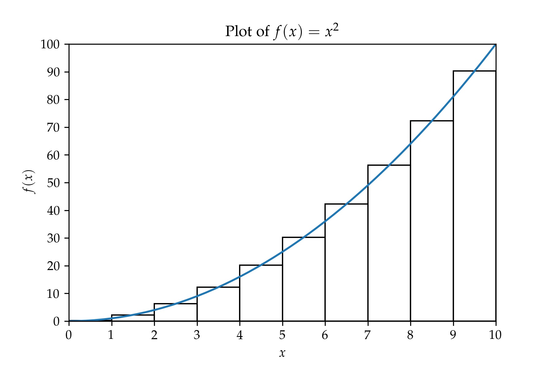
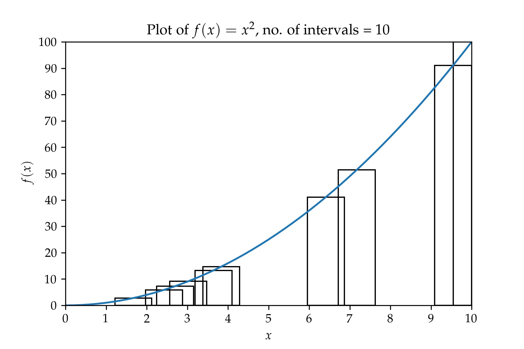
To make things concrete, let's consider a very simple integral $$I = \int_0^{10} x^2 \, \mathrm{d}x. \tag{1}$$ To get an estimate of the integral we can divide the $x$-axis into a number of equally sized intervals and then compute the sum of the areas of the rectangles whose heights are equal to the function values at the middle points of the intervals and whose widths are equal to the interval size. This is shown in the figure below for 10 intervals from $x = 0$ to $x = 10$ and for an interval size, $\Delta x = 1$. The greater the number of intervals, the smaller the interval size, and the more accurate the estimate of the integral.

In fact, this is the starting point for how the Riemann integral is defined—the Riemann integral of any function is equal to the area under the graph of the function. See chapter 7 of Understanding Analysis [1] for a more detailed understanding of how areas under curves, differentiation and integration are all related to each other.

Briefly, for a general function, $f(x)$, we define the integral from $a$ to $b$ by partitioning $[a, b]$ into an arbitrary ordered set $$P = \{a = x_0 < x_1 < ... < x_{n - 1} < x_n = b\}.$$ For each sub-interval $[x_k, x_{k + 1}]$ we define the infimums and supremums over those intervals $$m_k = \inf\{f(x) : [x_k, x_{k + 1}]\},$$ $$M_k = \sup\{f(x) : [x_k, x_{k + 1}]\},$$ and then compute the lower and upper sums over those partitions. $$L(f, P) = \sum_{k = 1}^n m_k (x_k - x_{k - 1}),$$ $$U(f, P) = \sum_{k = 1}^n M_k (x_k - x_{k - 1}).$$ Now, taking the set of all partitions $\mathcal{P}$ of the interval $[a, b]$, the integral $I = \int_a^b f(x)\,\mathrm{d}x$ is defined to be $$L(f) = \sup \{L(f, P) : P \in \mathcal{P}\}$$ $$U(f) = \inf \{U(f, P) : P \in \mathcal{P}\}$$ if $L(f)$ and $U(f)$ both exist and $L(f) = U(f)$.

Expressed in simpler mathematical notation the above definitions say, to the effect, that $$ \begin{eqnarray} I & = & \int_a^b f(x)\,dx \\ & = & \lim_{n \rightarrow \infty} \sum_{k = 1}^n f\left(\frac{x_k + x_{k - 1}}{2}\right) (x_k - x_{k - 1}). \tag{2} \end{eqnarray} $$ As $n \rightarrow \infty$, we have to fit more intervals in between $a$ and $b$ and so the delta between subsequent pairs of values $x_{k - 1}$ and $x_k$ has to get smaller. Additionally, the infimums and supremums both approach $f\left(\frac{x_k + x_{k + 1}}{2}\right)$ as $n \rightarrow \infty$.

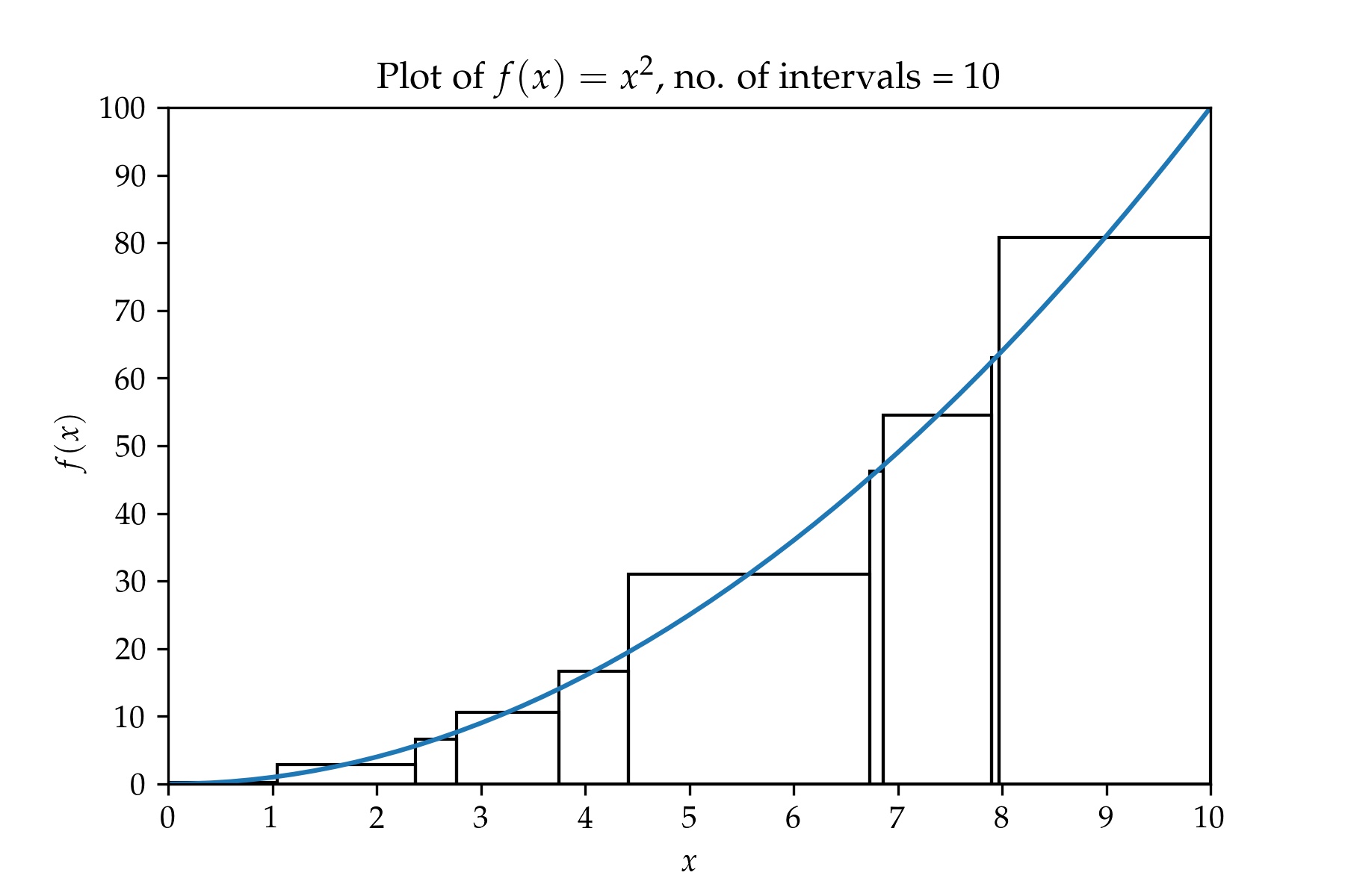
Note that the definition of the integral does not specify anywhere that the intervals should all be of equal size. Here is a plot of $f(x) = x^2$ with a partition containing 10 intervals.

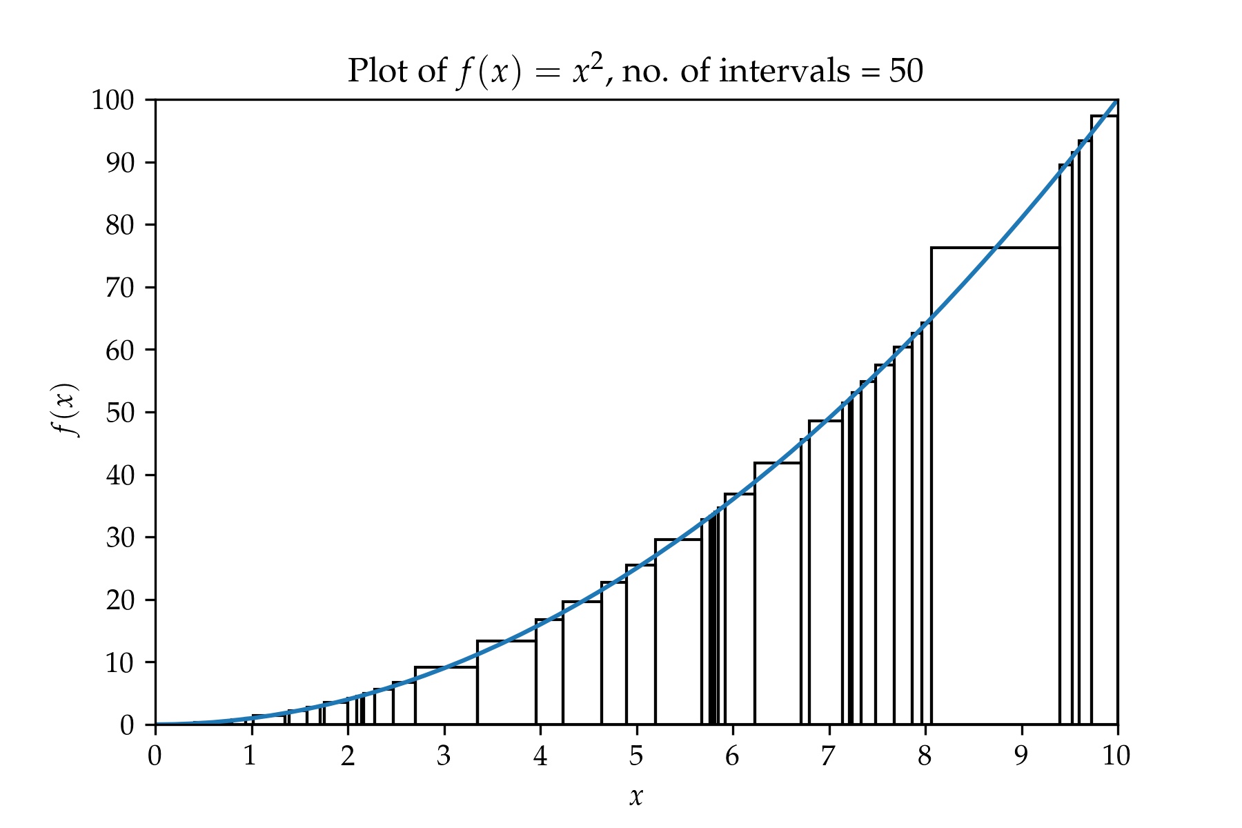
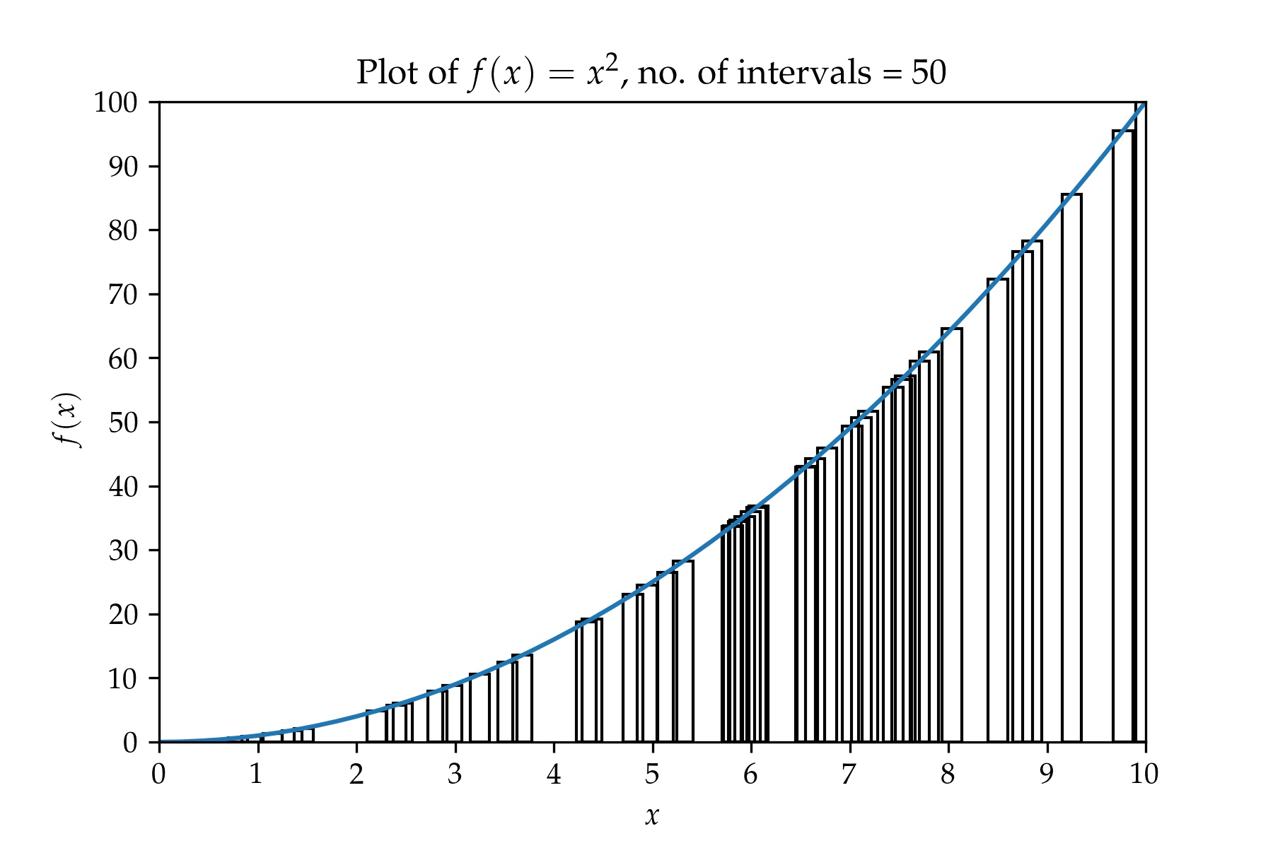
A plot containing a partition with 50 intervals.

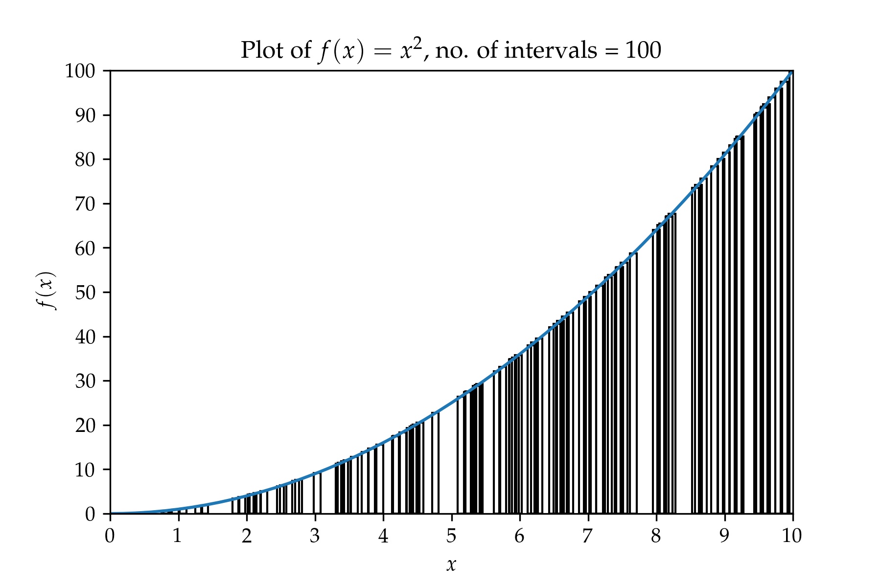
And a plot containing a partition with 100 intervals.

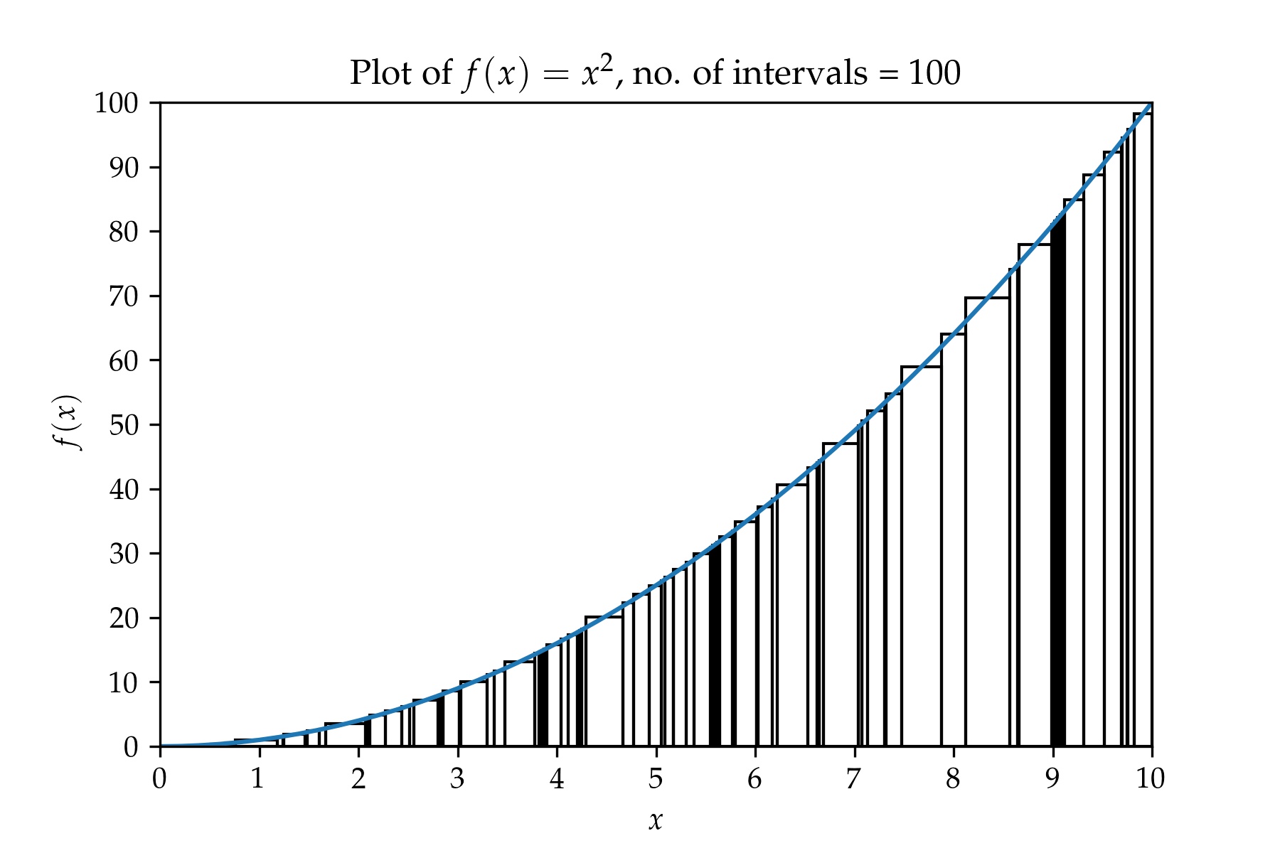
Looking at these plots it looks like we are taking a random sampling of points along the $x$-axis and then computing the sums of the areas of the rectangles whose heights are equal to the function values $f(x)$ at those randomly sampled points and whose widths are equal to the interval widths. There is one complicating factor here, the widths of the rectangles have to be chosen so that the rectangles do not overlap with each other. It would be nice to not have to worry about the widths of the rectangles—can the widths of the rectangles be made constant?

Let's return to equation 2 and see if we can still calculate the integral by randomly sampling the function $f$ in the interval $[a, b]$ while keeping the widths of the rectangles constant. The graphs we obtain as we increase the number of samples will look something like what's shown below. A plot containing a partition with 10 intervals:

A plot containing a partition with 50 intervals:

And a plot containing a partition with 100 overlapping intervals:

Do you see the difference when you compare the last three plots with plots 2, 3, and 4? The rectangles overlap with each other. But as we increase the number of samples, the widths of the rectanges get smaller and smaller. Can we take the limit and so make the overlap infinitesimal and hence calculate the integral? Let's try ...

Let's consider a uniform random variable $X$ whose values lie in the range $[a, b]$. We take $n$ samples, $\{x_k : k = 1 \ldots n \}$ and order the samples so that they form a partition of $[a, b].$ We now calculate the quantity $$I' = \sum_{k = 1}^n f(x_k) \Delta x$$ where $\Delta x = (b - a) / n$. Now let's rearrange the right hand side slightly. $$ \begin{eqnarray} I' = \sum_{k = 1}^n f(x_k) \Delta x & = & \sum_{k = 1}^n f(x_k) \frac{b - a}{n} \\ & = & \sum_{k = 1}^n \frac{f(x_k)}{\frac{1}{b - a}} \frac{1}{b - a} \frac{b - a}{n} \end{eqnarray}$$ If we recognize $\frac{1}{b - a}$ as the probability density function of $X$, then we can see that the term inside the sum is composed of the product of three terms :$f(x)/p(x)$, $p(x)$, and $\Delta x = \frac{b - a}{n}$. Now if we let $n \rightarrow \infty$ the rectangles we use to compute the area under the curve become infinitesimally thin and $I' \rightarrow I$. But from our studies of probability theory, we are also calculating the expectation value of $\frac{f(x)}{p(x)}$. So we can calculate the integral we want by simply calculating the expectation value of $\frac{f(x)}{p(x)}$.

Let's generalize this for any function $f(x)$ and any random variable $X$. Let $f:\mathbb{R} \rightarrow \mathbb{R}$ be any function and let $X:\omega \rightarrow \mathbb{R}$ be a random variable with probability density function $p(x)$. The expectation value of $f(x) / p(x)$ is given by: $$ \begin{eqnarray} \mathbb{E}\left( \frac{f(x)}{p(x)} \right) & = & \int_a^b \frac{f(x)}{p(x)} p(x) \, \mathrm{d}x \\ & = & \lim_{n \rightarrow \infty} \sum_{k = 1}^n \frac{f(x_k)}{p(x_k)} p(x_k) \Delta x \\ & = & \lim_{n \rightarrow \infty} \sum_{k = 1}^n \frac{f(x_k)}{p(x_k)} \mathbb{P}(X \in [x_k, x_k + \Delta x]) \end{eqnarray} $$ But for a given experiment, the probability that $\mathbb{P}(X \in [x_k, x_k + \Delta x])$ is simply $\frac{1}{n}$. So the right hand side becomes, $$\mathbb{E}\left( \frac{f(x)}{p(x)} \right) = \int_a^b f(x) \, \mathrm{d}x = \lim_{n \rightarrow \infty} \frac{1}{n} \sum_{k = 1}^n \frac{f(x_k)}{p(x_k)}. $$

[1] Stephen Abbott. Understanding Analysis. Springer, 2000.